Thursday, May 27, 2010

Fallacy in the Knappenberger et al study


This is a follow-up post to the previous post on the pending paper:

“Assessing the consistency between short-term global temperature trends in observations and climate model projections"

by Patrick  Michaels, Chip Knappenberger, John  Christy, Chad  Herman, Lucia  Liljegren and James  Annan


I'm calling it the Knappenberger study because the only hard information I have is  Chip's talk at the ICCC meeting. But James Annan has confirmed that Chip's plots, if not the language, are from the paper.

Fallacy is likely because, as I showed in the previous post, the picture presented there is considerably different after just four months of new readings. Scientific truth should at least be durable enough to outlast the publication process.

The major fallacy


Chip's talk did not provide an explicit measure of the statistical significance of their claim of non-warming, despite hints that this was the aim. The main message we're meant to take, according to James, is
"the obs are near the bottom end of the model range"
Amd that's certainly what the plots suggest - the indices are scraping against that big black 95% level. This is explicit in Chip's slide 11:
"In the HadCRUT, RSS, and UAH observed datasets, the current trends of length 8, 12, and 13 years are expected from the models to occur with a probability of less than 1 in 20. "

But here's the fallacy - that 95% range is not a measure of expected spread of the observations. It expresses the likelihood that a model output will be that far from the central measure of this particular selection of models. It measures computational variability and may include some measure of spread of model bias. But it includes nothing of the variability of actual measured weather.

The GISS etc indices of course include measurement uncertainty, which the models don't have. But they also include lots of physical effects which it is well-known that the models can't predict - eg volcanoes, ENSO etc. There haven't been big vocanoes lately, but small ones have an effect too. And that's the main reason why this particular graph looks wobbly as new data arrives. Weather variability is not there, and it's big.

Sources of deviation


I posted back in Feb on testing GCM models with observed temperature series. There were three major sources of likely discrepancy identified:

    Noise in measured weather
    Noise in modelling - unpredictable fluctuations
    Uncertainty from model selection


I showed plots which separated the various effects. But the bottom line is that the measured trends and the model population means both have variance, and to compare them statistically, you have to take account of combined variance (as in a t-test for means).

I railed against Lucia's falsifications of "IPCC projections" a couple of years ago. A big issue was that Lucia was taking account then of weather noise, but not model uncertainty. The result is that something that was then "falsified" is no longer false. The total variability had been underestimated. The same effect is being seen here in reverse (model noise but no weather noise).

Estimating model uncertainty


I don't know in detail how the probability levels on Chip's slides were calculated. But it's hard, because model runs don't form a defined population subject to random fluctuations. They are chosen, and with fuzzy ctiteria. Individual runs have fluctuations that you can estimate, but there's no reason to suppose that across models they form a homogeneous population.

That is significant when it comes to interpreting the 95% levels that are quoted. As often in statistical analysis, there's no real observation of the tail frequencies. Instead, central moments are calculated from observation, and tail probabilities quoted as if the distribution is normal.

Normality is hard to verify, and even if verified for the central part of the distribution, it's still a leap to apply that to the tail. The unspoken basis for that leap is some variant of the law of large numbers. If getting into the tail requires the conjunction of a number of independent happenings, then it's a reasonable guess.

But if the occurrence of a tail value is dependent on simple selection (of model run), then even if the scatter looks centrally bell-shaped, as in Chip's slide 5, the reasons for thinking the tail fades away as quickly as a normal distribution would is not really there. The slide does note correctly that the points on the histogram are not independent.

Tuesday, May 25, 2010

What a difference four months makes!


Deep Climate, at Tamino's, noted one of the interesting talks at the ICCC meeting was by Chip Knappenberger. It foreshadows a paper submitted to GRL by an eclectic group of authors:

“Assessing the consistency between short-term global temperature trends in observations and climate model projections"
by Patrick Michaels, John Christy, Chad Herman, Lucia Liljegren and James Annan

I presume Chip is an author too, although it isn't entirely clear. Anyway, he shows some plots, apparently from the paper, of temperature trends measured back from present to periods of from five to fifteen years. These are compared with model predictions, with the general idea of suggesting that they have been overpredicting warming. In fact, the talk pauses a couple of times to examine the phrase, written in very large font:
"Global Warming has Stopped!”

Global warming has stopped (or at least greatly slowed) and this is fast becoming a problem.

Present for this paper means end 2009. So I thought it might be interesting to update with four months more data.

(Updated discussion below)


Here are the two relevant slides from the talk. They split into land instrumental and satellite:


And here are my updates, moving the starting point forward four months. I haven't seriously tried to calculate the probability bounds - they just roughly follow the original for visual comparison. Following Carrot Eater's suggestion, the plot is animated, with the higher value using the more recent data


Update: 
The new data shows that:
1. GISS trend is positive in the range
2. Hadcrut3 is weakly positive
3. NCDC is mixed
4. UAH is quite positive
5. RSS is mixed
Not really a basis for concluding that warming has stopped. And after a few more months of warmth....?

Looking forward

To see what the plots might look like by end 2010 (when this paper might appear), I calculated the same trend diagram assuming that each coming month, for each index, was as warm as April 2010. Here are the plots, with the old trends shown as thinner curves:


As you'll see, not only are all trend curves decidedly positive (warming) but getting close to the central value of the models.

Sunday, May 9, 2010

The Greenhouse Effect and the Adiabatic Lapse Rate


This post is prompted by recent posts by Steve Goddard on WUWT about the GHE and the lapse rate on Venus. They muddle the effects, in a way that is quite often seen in the blogosphere. The meme is that surface warming is due to the lapse rate and not to the GHE. Often on WUWT this comes down to even more simplified assertions that warming is due to atmospheric pressure.

The fact is that the dry adiabatic lapse rate, and the mechanism that creates it, are an intrinsic part of the greenhouse effect that causes warming at the surface. More below the jump.


The elementary GHE explanation


A brief explanation of the GHE usually notes that the atmosphere is differentially transparent, letting most sunlight through, but obstructing IR. This is described as trapping heat, or blanketting or whatever.

This sometimes is criticised for inexactness. It's true that the heat isn't trapped - it all gets out. And a blanket isn't quite right.

Still, the reasoning does reliably lead to the right answer. With physical situations, where there is a flow driven by siome kind of potential and the flow is impeded in some way. the potential builds up behind the impedance. It has to, in order for the flow to get through. It happens with electrical circuits, river flows, even in economics. But it's true that more can be said about the mechanism.

The dry adiabatic lapse rate


I posted a while ago on the dry adiabat and the atmospheric heat pump which maintains it. Any gas in motion in a gravity field will have a vertical component to the motion. When it moves down or up, it is compressed or rarefied. Respectively, it is heated or cooled. This heat change then diffuses in to the gas at the new level. Both up and down motions have the effect of pumping heat downward, until the dry adiabat lapse rate is achieved. This is a temperature gradient, warming in the downward direction, and the critical level is g/cp, where g is the acceleration due to gravity and cp is the constant pressure specific heat of the gas.

As I said, maintaining such a gradient requires a heat pump, because heat tends to move down the gradient by conduction. The energy for the pump comes from atmospheric motions, which are thus attenuated. But when a large heat flux is passing through the air, as in the solar flux which causes all kinds of differential heating, there is energy to drive and sustain these motions. And because the energy sink is the need to overcome conductive leakages, the drain is small, because, the conductivity is low (although there are other demands too).

Adiabat, solar flux and no GHG


Suppose then we have an atmosphere of nitrogen, which does not absorb or emit IR. Sunlight is converted to heat at the surface, and to maintain energy balance, this heat must be radiated back to space.This goes straight through the N2. The surface will warm to just the temperatrure that is needed, on average, to achieve that outward radiation level.

The surface will not be uniform. Some parts will be hotter than others, and this will set up local convection cells. Bigger cells will take heat from the tropics to colder parts. The N2 will be in motion.

So, I hear you say, shouldn't the energy balance include convection from the surface. Well, there will be some exchanges, but on balance, heat flux to the N2 goes nowhere. For N2 cannot emit it to space. It can only conduct it back to the surface (somewhere).

The important thing to note is that the dry adiabat has nothing to do with IR properties. It only requires gravity and motion. The N2 atmosphere will have that g/cp gradient. But it will start from the surface temperature fixed by the IR balance, and get colder as you go up.

Snowball Earth


An example often cited is of the Earth without GHG's. To keep in balance with sunlight, after allowing for albedo, the Earth has to emit about 235 W/m2. At a uniform surface, the temperature required to do this is about 255K. This is much less than the temperatures we have, and the difference of about 33K is ascribed to the greenhouse effect.


Greenhouse gases


When there are GHG's that absorb and emit IR, there are many changes. One thing that doesn't change, though, is that the heat absorbed from the Sun must still get out to space. The question is what warming will occur to make that happen.

One thing that does change is what actually emits the heat. GHG's, like surfaces, emit according to their temperature. At many wavelengths, the main GHG's, H2O and CO2, are dense enough to absorb nearly all the IR emitted from the surface. Kirchhoff's Law says that, at each wavelength, emissivity equals absorptivity. So at these absorbing wavelengths, water and CO2 are also the main sources of emission that go out to space. At other wavelengths (the atmospheric window), the emission to space is direct from the ground.

But the absorption and emission happen at different places. Much of the IR is absorbed soon after leaving the ground. At those frequencies, IR is also emitted from the same gases high in the atmosphere. The absorption and emission are not directly connected. The heat absorbed has to somehow reach those upper levels before emission can occur. That is another interesting story.

The adiabat and heat balance


Meanwhile, the adiabat is still there. It is determined by the properties of the non-GHG gases (at least on Earth). And it ensures that the emission from GHG occurs at a much lower temperature than the surface.

For the adiabat, I've used the analogy of a battery, which maintains a voltage difference between its ends of, say, 1.5V, but does not determine the actual voltage there. That depends on how it is "earthed". In the non-GHG case, it is "earthed" at the ground, where the temperature is fixed by radiation balance. Since no "current" (heat flux) flows through the battery at the top, it's voltage is just 1.5V less, passively determined.

When emission occurs from GHG's at TOA, a similar heat balance equation determines the temperature there. That is where the adiabat "battery" is "earthed". The temperature gradient below is still fixed, and hence so is the surface temperature - at a much higher level. That is the complete greenhouse effect.

So for the Earth?


If GHG's had uniform strong effect over IR frequencies, then the whole 235 W/m2 would be emitted from TOA, and this would have to happen at the snowball earth temperature of 255K, on average. TOA for this purpose is probably about 10 km or more, so the Earth's surface would be about 355K. very hot. The actual location of the emission depends on the GHG concentration. If it is lowered, some of the emission will come from lower levels, reducing the average height, and hence the temperature at the surface.

It should be said too, that on Earth the dry adiabat is rarely attained. That is mainly because the air is not dry, and water phase changes reduce the gradient considerably.

In fact, as I've mentioned, the Earth has an atmospheric window, through which some of the IR (about 40 W/m2) is emitted with a spectrum corresponding to the warmer ground surface. That leaves less to be emitted at the top, and so the temperature can be lower. Indeed, the effective emission from GHG's is at about 225K - so instead of a uniform 255K emission temp, we have part at about 288K and part at about 225K. That reduces the ground temp by about 30K.

Spectra


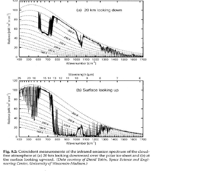
You can see how this works for the Earth from observed spectra. Below is a plot of IR spectra observed near Barrow, Alaska (source , from Grant Petty's textbook "A First Course in Atmospheric Radiation"). The top plot shows , in effect, outgoing IR. It's only part of the thermal spectrum, but shows a dip between 600 and 800 cm^-1, which is emission from CO2, and to the right of that, the atmospheric window, where IR comes largely unimpeded from the surface. Note that in the dip it tracks the BB curve for about 225K, and in the window, about 268K - the spectrum is taken over a polar ice sheet near Barrow AK. The lower plot shows the IR reaching the surface below. Corresponding to the emission CO2 dip above, there is a peak caused by atmospheric (low level) CO2 emission.


Saturday, May 8, 2010

Scale of spatial correlation

I've been trying to follow up on the discussion here of whether the Hansen/Lebedeff claim of correlation of temperatures (longterm) over 1200 km is reasonable. I mentioned kriging as one line to follow.

Kriging is a method for interpolating from a rather random distribution of spatial information. The original application was to mining and borehole information.

You have a spread of readings and would like to know something about the mineral field in between. You'd probably like to know where to drill next, You want a weighted formula which takes account of the fact that the further away the readings are, the more likely they to be influenced by just random noise. You want to balance the desire for a lot of readings with the need to value closer information more highly.

In R there's a kriging routine in the package geoS. But it seems to be oriented to distribution of a single variable, whereas we typically have a time series at each point. In mineral exploration, a reasonable analogy is a core profile, and there must be stuff for that.

Or I could try just using trend as the single variable. A problem there is that we don't have a uniform trend period.

Kriging depends on estimation spatial correlation, and this is often done by fitting parameters of a variogram. This rather comes back to the weighted average idea climate people use. For example, GISS uses a linear taper weight function, held at zero beyond the bounding radius, which could be regarded as the parameter.

There are a number of commonly used functions for variogram fitting, of a generally Gaussian shape. This conical function, with its discontinuous derivative, is not one of them, and with good reason. The fitting algorithms usually involve minimising with derivatives.

Anyway, I thought I'd at least do some exploratory analysis varying the radius. Details below the jump.


I began by looking at Kansas City - surrounded by lots of land stations. I soon found that Leavenworth, nearby, had a better record, so I used that.

I looked at distances of 1200, 800, 500 and 200km. Using the GISS conical weighting, I tried to see how the interpolated temperatures matched each other, and the measured temperature.

Firstly some maps, to show how many stations are involved, at the various radii. They give an optimistic view, because numbers drop off in recent years, and especially since 2005. So I've stopped the graphs at 2005.

1200 km

800 km

500 km

200 km

Now here are the plots, on a single graph. You'll see that they do converge, and the 1200 km is noticeably out of line with the others, but not extremely so. What is out of line is the Leavenworth measurement (in black).

What that suggests to me is that the generally idea of homogeneity adjustment has some merit. It seems clear that the central measure tracks for some periods, jumps, and then tracks some more, which is just what the homogeneity test is designed to fix.
And here are the trends:

Trend Leavenworth 1200km 800km  500km  200km
Number 1 96848021935
1901-2005 -0.02 0.013-0.01-0.009-0.016
Trend_se 0.030.020.020.020.03
1979-2005 0.720.240.260.190.09
Trend_se 0.220.130.160.160.19

Saturday, May 1, 2010

Just 60 stations?.

Eric Steig at Jeff Id's site said that you should be able to capture global trends with just 60 well-chosen sites. Discussion ensued, and Steve Hempell suggested that this should be done on some of the other codes that are around. So I've given it a try, using V1.4 of TempLS.

I looked at stations from the GHCN set that were rural, had data in 2009 2010, and had more than 90 years of data in total. The selection command in TempLS was
"LongRur" = tv$endyr>2009 & tv$length>90 & tv$urban == "A",
That yielded 61 stations.

Update: This topic was revisited  here

Results and comparisons below the jump.

A summary of this series of posts is here.


First a map of the 61 stations. I've called the station set "LongRur":
First comparison is with the Hadley land-only CRUTEM3, annual and smoothed with the IPCC AR4 Chap 3 13-point filter. Note that the dates are wrong in the titles - the plot is actually 1902 to 2009.


Much more annual fluctuation, but the smoothed curves track well.

And here is GISS Land only:

Now a comparison of the inferred temperature with GISS Land/ocean. This and the next are less direct analogues, because of the inclusion of ocean temperatures.

Here is a comparison with HadCrut3 (land/ocean):
Clearly the smaller set has greater excursions. But it's true that the trend looks much the same, although the 61-station set rises more rapidly towards the end. That is expected when comparing a land station set  (with several oceanic islands)  with a land/ocean trend. I'll post comparative numbers later.(trends are below)


Here are the plots of the TempLS outputs with trends and a smooth, over two time periods:

Trend Comparison

Here are the linear trends, 1902 to 2009, in deg C/Decade
LongRur     CRUTEM3  Giss          HadCRUT
0.0860.087  0.0690.076
The match to the land-only trend (CRUTEM3) is  very good.